Process plants hold years of operating history, yet much of their control still runs on linear models tuned for a narrow operating window. Reinforcement learning (RL) takes a different route. A controller learns its policy from experience and can weigh margin, reliability and emissions in the same decision. This article explains how RL works in a plant and where it applies: closed-loop process control, maintenance scheduling and energy management.
How reinforcement learning works
Traditional control designs depend on a precise mathematical model of the process. Reinforcement learning frames control as a Markov Decision Process (MDP). The agent observes the state of the process, chooses an action, receives a reward, and learns a policy that maximizes the cumulative reward over time.
The agent does not have to learn on the live process. It can explore and improve control strategies against a model of the environment instead. In a plant, that means training offline on an accurate representation of the unit's behavior, without disrupting operations or adding risk. That matters most in complex, multivariable units, where trial and error on the real process is not an option.
Done this way, RL can improve throughput, energy efficiency and margin with fewer manual adjustments, while operators keep authority over the unit. Common objections, such as whether a data-first model leaves out first principles or needs frequent retraining, are taken up in myth busters: reinforcement learning in closed-loop control.
1. Real-time process control
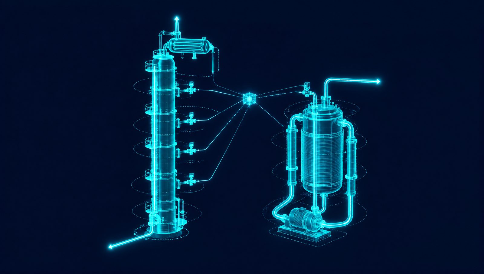
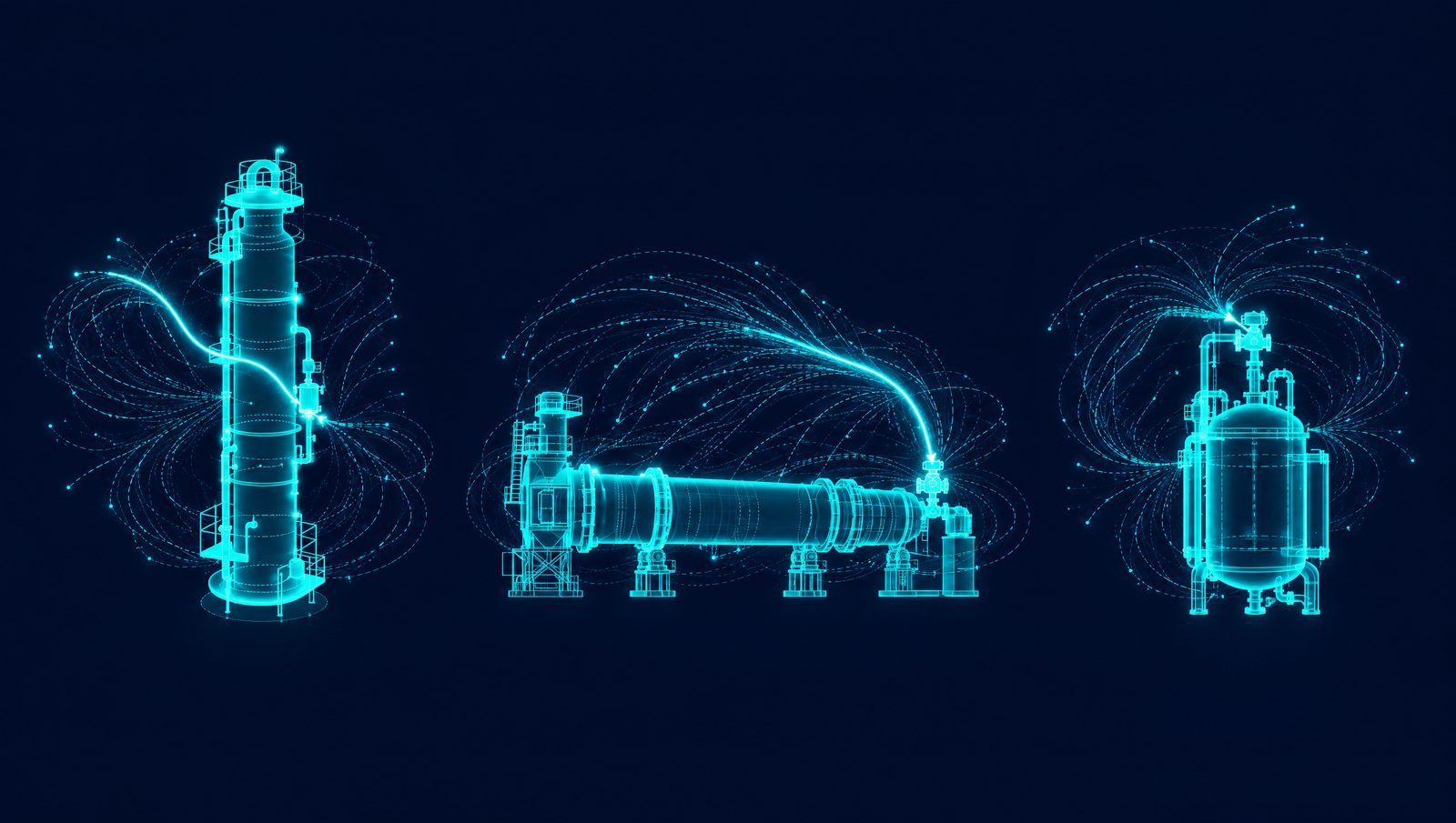
Fractionators, kilns and reactors are nonlinear and multivariable, and that is where conventional advanced process control (APC) reaches its limits. An RL controller does not need a perfect first-principles model. It learns its policy against a dynamic model of the unit trained on the plant's own operating history, which captures the nonlinear behavior linear models miss.
Once deployed, the controller reads the current state of the unit and responds to shifts in feed quality, catalyst activity or ambient conditions as they appear. Fresh plant data keeps the underlying model current as the unit changes. Because the controller writes setpoints through the existing control layer to the distributed control system (DCS), the plant keeps its APC and needs no new hardware.
Transparency matters as much as performance. When engineers can see how the model expects the unit to respond and why the controller chose a move, the concern that a neural network is a black box can be tested directly against the unit's behavior.
How a deployment proceeds
- Map the data. Historian and DCS tags are mapped so the model can take in high-frequency operating data. Gaps are filled with inferentials built from established equipment correlations.
- Train in simulation. The RL agent explores a wide range of scenarios offline and learns the safe operating envelope before it adjusts a live valve.
- Review and constrain. Engineers review the candidate policy, set the economic and safety constraints, and approve promotion to advisory mode, where operators review each recommended move.
- Close the loop. The controller calculates setpoints and writes them to the DCS, always within the boundaries the plant has defined. Operators keep the authority to override any move.
The result is a self-optimizing layer above APC that holds the unit closer to its economic targets for throughput, fuel and yield as conditions change, and frees the team for higher-value work.
2. Predictive maintenance
Conventional predictive maintenance reacts to patterns or anomalies in equipment data. A reward-based approach goes a step further and optimizes the maintenance schedule itself, weighing uptime against the cost of disruption.
Models trained on sensor data and simulation learn how equipment degrades. That is useful in applications such as compressor health monitoring and grinding-mill uptime. Anticipating failure allows planned maintenance in place of emergency repair, which reduces unexpected outages, supports spare parts planning and extends the life of capital-intensive equipment. Scheduling from real-time condition data, instead of a fixed calendar, keeps maintenance windows short and placed where they disrupt production least.
In mining and minerals, where grinding-mill availability often limits how much ore the plant can process, condition-based scheduling helps hold both safety and production.
3. Energy management
Cutting energy cost without missing production targets is a trade-off an RL agent can be designed to make. The agent weighs power prices, emissions limits and process constraints against throughput objectives, and selects the control moves that meet those objectives at the lowest energy cost per unit of product.
The reward function is where cost and sustainability meet. Energy saved earns a positive reward, and excess emissions carry steep penalties. That teaches the agent to favor actions such as adjusting furnace temperatures, retuning motor speeds or shifting load to on-site renewables, which keep the plant inside its budget and emissions limits.
Because the policy responds to the current state, it adapts when power tariffs spike or process conditions drift, without constant manual retuning.
How Imubit applies this
The Imubit Platform's Deep Learning Process Control® (DLPC®) pairs a Deep Learning Predictor, which learns a nonlinear dynamic model of each unit from its own history, guided by first principles, with a Deep Learning Controller trained by reinforcement learning across millions of simulations. In Imubit's Map, Model and Control, the predictor carries the Model step and the controller carries the Control step. The controller runs on-premise and writes setpoints to the existing APC or DCS minute by minute, inside limits set by plant engineers. Imubit has over 100 closed-loop controllers deployed worldwide, the largest install base in the industry, and works across refining, chemicals and polymers, cement, and mining and minerals. Read more about the technology.