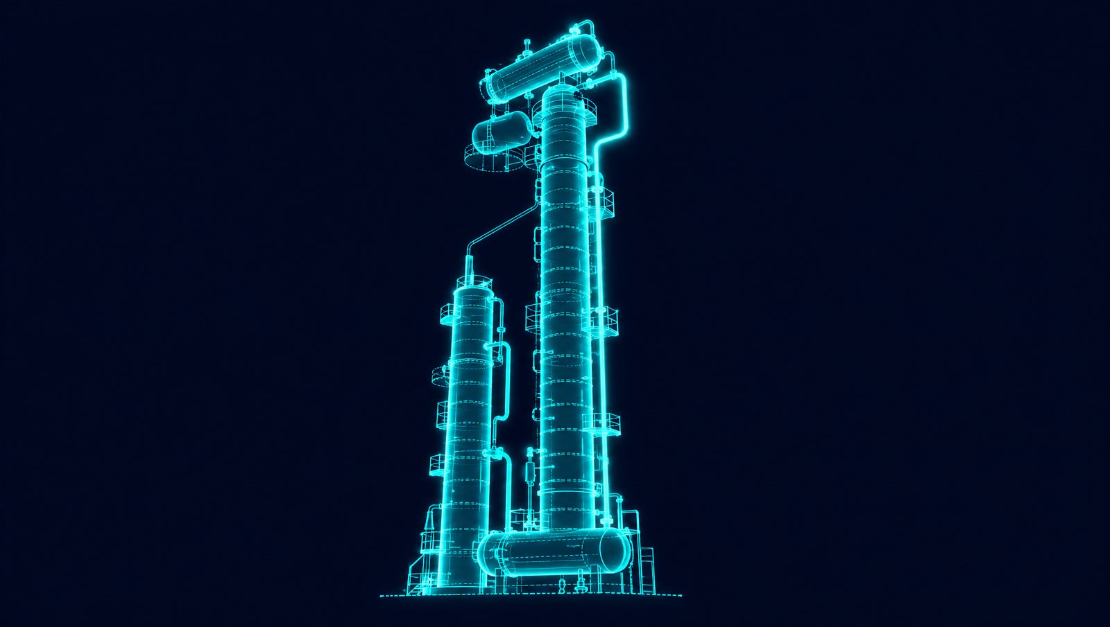
Propylene recovery looks straightforward on paper. In practice the propane/propylene (C3) splitter is one of the most energy-intensive columns in the complex. Propane and propylene boil close together, so the separation needs a tall column with many stages and high reflux, and that drives steam demand and operating cost. Every feed swing costs recovery, purity or steam.
When volatile feedstock prices and logistics disruptions squeeze margins, small inefficiencies in this unit add up. Conventional control models struggle with it, because the relationships among pressure, temperature, reflux and feed composition are nonlinear and shift with conditions. A model learned from the unit's own data can follow those relationships and steer setpoints to maximize recovery while using less energy. The six steps below show how to get there.
Prerequisites: is the unit ready?
Before building any model, confirm you can feed it quality data. High-frequency data from the key equipment, including towers, exchangers and compressors, matters most. A full twelve months of history is not strictly required before model development begins.
Gaps and noisy streams weaken any algorithm. Confirm that the process historians hold second- or minute-level data, and check their compression settings, since historian compression can introduce small losses.
A robust distributed control system (DCS), backed by stable PID loops and an advanced process control (APC) layer, provides the execution. Without it, a model can recommend but cannot act. Once closed loop begins, setpoints have to be written safely and predictably through that layer.
Use this checklist to judge readiness:
- Sensor health and recent calibrations
- Lab sample frequency matched to the process dynamics
- Historian tag latency below a few seconds
- Firewalls configured for secure data bridges
- IT/OT connectors that expose real-time data to the optimization platform
- Enough on-premise compute, or a secure edge, to run the model without interrupting critical operations
Well-documented tags give operators the transparency they need to trust the model. Quick fixes such as recalibrating drifting transmitters, flagging stale lab tags and tightening historian deadbands often add more value than new hardware.
Step 1: Benchmark current performance and data quality
Pull high-frequency data from the DCS historian at short sampling intervals, and trim out shutdowns and turnarounds. From that clean slice, calculate baselines for propylene recovery, reboiler steam per tonne and unplanned downtime hours. Heat maps and box plots show feed-swing bias and other patterns that dilute recovery.
Scoring each tag from 0 to 5 for completeness, accuracy, resolution and latency is a useful internal heuristic, though it is not a formal standard in process data validation. A single unreliable flow meter can skew the model. Robust baselines depend on reliable historians, and poor data quality will undermine a closed-loop effort before it starts.
Step 2: Define objectives and success metrics
Before modeling, decide what success looks like for the unit. Translate corporate goals into targets the control room can track, such as a gain in propylene recovery, a cut in reboiler steam per tonne or a tighter cushion on product purity.
Attach economics to every target. Use the planners' latest price set so the model can convert each extra kilogram of propylene, or each kilogram of steam saved, into margin. Linking objectives to real economics keeps everyone focused when feedstock prices move with regional logistics.
Fix a baseline window of steady operation before the model goes live, long enough to capture the unit's normal variability, and keep the same KPI definitions afterward. Statistical tests such as a t-test then show whether improvements exceed natural variability. A fixed, agreed baseline prevents later debate about shifting goalposts.
Align operations, planning and leadership. Daily huddles that show how each control move supports the splitter's energy-intensity targets connect decarbonization goals with front-line action. Higher recovery at lower steam per tonne also lowers emissions intensity.
Step 3: Integrate and monitor data
Connect the DCS and process historians to the optimization platform through open protocols such as OPC UA or MQTT. High-frequency tags stream directly to the platform, so small pressure changes in the splitter and short feed swings are captured. Then build a single tag dictionary. Reconciling "C301_P" and "C-301_Press" into one standard name prevents model blind spots and speeds later troubleshooting.
Clean data is the foundation. Automated routines remove deadband artifacts, flag slow drift and align lab results with online measurements. That cleaning has to run continuously, because a model that learns from bad inputs will push the column in the wrong direction. Even well-maintained historians hold idle tags and sampling gaps that need to be removed before training, or the errors carry through every layer of the optimization.
Configure live dashboards that show propylene recovery, steam rate and anomaly alerts in real time. If operators cannot see the KPI the model is optimizing, trust erodes quickly.
Three integration problems come up often:
- Firewall rules often block MQTT traffic. Open just the required ports to keep the cybersecurity posture intact.
- Inconsistent tag conventions cause confusion later. Batch-rename with a script before ingestion instead of retrofitting names.
- Lab delay throws off the models. A rolling buffer that shifts sample timestamps to match process time corrects for it.
Step 4: Build predictive and control models
Map every variable that influences the splitter: tower pressure, top temperature, reflux ratio, feed olefin content, steam flow, condenser duty and even ambient humidity. A complete feature list lets the model see the same details that operators watch on the DCS.
A practical approach combines mass and energy balances with deep learning. The physics keeps predictions grounded, and the network learns the nonlinearities that conventional control struggles with.
After cleaning, split the data into training, validation and test sets, and use cross-validation and early stopping to catch overfitting. That discipline keeps the model reliable when feed composition or ambient conditions change.
Transparency matters for operator confidence. Sensitivity views such as SHAP plots and tornado charts show how a one-kilopascal pressure change moves recovery, or which steam trims return the most.
Step 5: Move to closed loop
Start in advisory mode. The model observes the unit and surfaces recommended setpoints without writing to the DCS. When the recommendations match or improve on operator judgment, move to operator-approved moves, and then to closed loop, inside limits set by plant engineers.
Where the controller is trained with reinforcement learning (RL), it learns a policy for responding to feed swings and ambient shifts and acts on them as they happen. The existing APC stays in place. The optimizer moves manipulated variables inside the existing limits, and operators can override it at any time.
Before cutover, validate every tag path, add soft limits for unreliable I/O and run joint training sessions with the operators. These steps build trust and make the transition predictable.
Step 6: Validate, sustain and scale
Once the system is writing setpoints, compare the frozen baseline with an equal period of post-deployment data. A t-test at 95% confidence on the key indicators (propylene recovery, reboiler steam per tonne and unplanned downtime) shows whether the gain is real and not noise. Historian data makes those checks fast and transparent, which builds operator trust in the results.
Sustaining the value takes discipline. Retrain the model on a regular cadence and re-validate the economics periodically, so it follows drift in feed characteristics, upstream catalyst age and ambient conditions. Monitoring dashboards flag data gaps, and refresher training keeps operators confident enough to act on the model's moves.
With the splitter running well, turn to the next constraint. Depropanizers, debutanizers, ethylene fractionators and the FCC main fractionator often share utilities and constraints with the PRU. Optimizing them in sequence lets the combined models cover more of the separation train, so those shared limits are managed across the units together rather than column by column.
How Imubit applies this
Imubit applies Map, Model and Control to propylene recovery in refining and petrochemicals. Map traces lost recovery and excess steam to the recurring decisions behind them, such as splitter pressure, reflux and reboiler duty. Model learns the splitter's nonlinear dynamic behavior from its own history with Deep Learning Process Control® (DLPC®), guided by first principles, and a controller trained by reinforcement learning across millions of simulations learns the control policy. Control takes those decisions to closed loop, writing setpoints to the existing APC or DCS, inside limits set by plant engineers.